Conditional formatting #DIV/0! within Excel is easy enough, but that doesn't work in Pivot Tables.
Luckily, there's an option within Pivot Table options that allows you to configure what appears when an error value is raised.
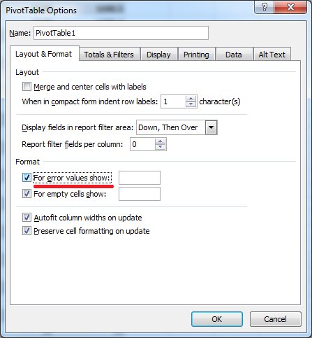
Hide Div 0
Simply check For error values show: and, in my case, leave the entry blank. Or set it to 0. Whatever works best for you. Divide by zero be gone with you.
Hope this helps!
I'm an Australian Chief Analytics Officer passionate about data science, visual insights, and all things sport—particularly cricket. An adventurer at heart, I’ve gone from abseiling cliffs to snorkeling in crystal-clear waters, sleeping in the wilds of Africa, and exploring destinations worldwide, with my latest trip taking me to Bali. When I'm not diving into data or analytics, I'm spending time with my three sons and two daughters, attempting to hit sixes for my local cricket club, reviewing chicken schnitzels or honing my craft around a coffee machine.


Sounds like such an easy solution. I’ve been using pivot tables for years, and I never noticed that little check box!!! Thanks!!!
Yeah mate, easier than it should be! 🙂 Or something like that. A hidden in plain sight gem that one.
Good tip, Mike.
Error values are an indication of something wrong, so it’s often good to check the source data to see why it’s happening. If the error is the result of an otherwise good formula, then IFERROR can hide them at source and the pivot table will show a blank.